Hubway Our Way: Exploratory Data Analysis on Hubway Trips 2015
I like cycling, so I wanted to do some data analysis on cycling. And then, what? The problem is I didn’t have any personal data about my trips (I don’t record my trip on Strava). Although I know, I commute 6 miles almost everyday or ~ 44 minutes on average / day. So, I decided to make something else but still about cycling.
Then I remember I live in Boston! (Uh, Ok…). In Boston, not only we have Red Sox but also Hubway. Hubway is bike sharing program in Boston, Cambridge, Somerville and Brookline area. Hubway publishes its trips data each month and contains the origin and destination, trip duration, gender, age and its user category. Great! Now I can work on a topic that interests me.
In doing data analysis, we first have to tidy the data, transform it, and visualize it. I won’t model it this time, what we will do is just exploratory data analysis (EDA).
Tidying and transforming the data
We are lucky, the dataset is already tidy. By tidy, I mean, every row represents a single observation, and every column represents a single variable. What remains, is just how we handle the missing values.
# We read the hubway data and combine them into one
# In the dataset there is characters \N to mark the empty data, we will replace
# them as NA.

hubway <- rbind(
  read_csv("201501-hubway-tripdata.csv", na=c("\\N")),
  read_csv("201502-hubway-tripdata.csv", na=c("\\N")),
  read_csv("201503-hubway-tripdata.csv", na=c("\\N")),
  read_csv("201504-hubway-tripdata.csv", na=c("\\N")),
  read_csv("201505-hubway-tripdata.csv", na=c("\\N")),
  read_csv("201506-hubway-tripdata.csv", na=c("\\N")),
  read_csv("201507-hubway-tripdata.csv", na=c("\\N")),
  read_csv("201508-hubway-tripdata.csv", na=c("\\N")),
  read_csv("201509-hubway-tripdata.csv", na=c("\\N")),
  read_csv("201510-hubway-tripdata.csv", na=c("\\N")),
  read_csv("201511-hubway-tripdata.csv", na=c("\\N")),
  read_csv("201512-hubway-tripdata.csv", na=c("\\N"))
  )
hubway <- as_tibble(hubway)
Here, we want to only focus with the trips under 30 minutes. Why? Because trips under 30 minutes won’t be charged extra. Who wants to pay extra?
# Tripduration is in second
# We also do mutate to get the age of each user
under_30_min_trips <- as_tibble(
  hubway %>%
  filter(!is.na(`birth year`), tripduration <= 1800) %>%
  mutate(age = 2015 - `birth year`)
  )

# Gender is represented by 0,1, and 2 here.
# To make it clear we change it into factor
under_30_min_trips$gender <- factor(under_30_min_trips$gender)
levels(under_30_min_trips$gender) <- c("Not Provided", "Male", "Female")
Exploratory data analysis
Exploratory data analysis starts with generating at least a question, confirming by visualizing the data, and then generate more questions based on the visualization. Now, as a start, we want to know whether people really usually ride under thirty minutes?
hubway %>%
  group_by(usertype) %>%
  summarise(p = mean(tripduration <= 1800)) %>%
  ggplot +
  geom_bar(aes(x = usertype, y = p), stat = "identity") +
  scale_y_continuous(labels=scales::percent) +
  labs(x = "User", y = "% of people who ride under or equal 30 minutes") +
  coord_flip()
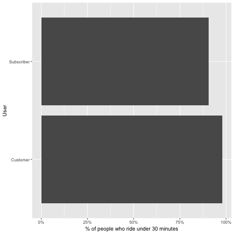
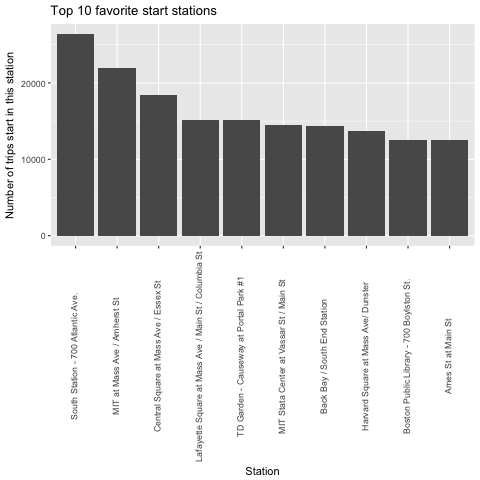
Now that we know more than 80 % of the trips are less than or equal 30 minutes. Next question we want to answer is: What is the most favorite route for trips under 30 minutes? We will try to see what is the most popular starts and destinations.
# Here we want to know which station is the most popular for start.
# We will just show the top ten for clarity in the graph
under_30_min_trips %>%
  group_by(`start station name`,
  `start station longitude`,
  `start station latitude`) %>%
  summarise(n = n()) %>%
  arrange(desc(n)) %>%
  head(10) %>%
  ggplot() +
  geom_bar(aes(
    x = reorder(`start station name`, desc(n)),
    y = n),
    stat = "identity") +
  theme(axis.text.x = element_text(angle = 90, vjust = .3)) +
  labs(x = "Station", y =  "Number of trips start in this station") +
  ggtitle("Top 10 favorite start stations")


# And which one is the most popular as destination
# We will just show the top ten for clarity in the graph
under_30_min_trips %>%
  group_by(`end station name`,
  `end station longitude`,
  `end station latitude`) %>%
  summarise(n = n()) %>%
  arrange(desc(n)) %>%
  head(10) %>%
  ggplot() +
  geom_bar(
    aes(
      x = reorder(`end station name`, desc(n)),
      y = n),
    stat = "identity") +
  theme(axis.text.x = element_text(angle = 90, vjust = .3)) +
  labs(x = "Station", y =  "Number of trips end in this station") +
  ggtitle("Top 10 favorite destination stations")
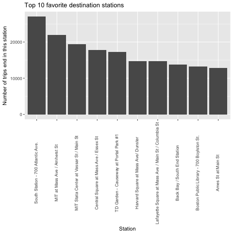
The graphs above don’t tell us what is the most popular route, because if we combine those two graphs, we will see that the most popular route starts and ends with the same station, which is not possible for a route.
under_30_min_trips <-
  unite(under_30_min_trips,
  route,
  `start station name`,
  `end station name`,
  sep = " to ")

under_30_min_summary <- as_tibble(
  under_30_min_trips %>%
  group_by(
  route,
  `start station longitude`,
  `start station latitude`,
  `end station longitude`,
  `end station latitude`
  ) %>%
  summarise(avg = mean(tripduration), n = n()) %>%
  arrange(desc(n))
  )

# Top ten short routes
under_30_min_summary %>%
  head(10) %>%
  ggplot +
  geom_bar(
    aes(
      x = reorder(route, n),
      y = n),
    position = "stack", stat = "identity") +
  labs(x =  "Number of trips", y = "Routes") +
  coord_flip() +
  ggtitle("Top ten routes")
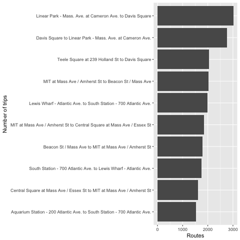
That represents what we are looking for, that is, the most favorite route for short trip is from *Linear Park to Davis Square**.
Now, let’s move on to the next question we want to search the answer: When is most of the Hubway user use the service in the year?
# Usage each month
under_30_min_trips %>%
  ggplot(aes(x = as.Date(starttime))) +
  geom_histogram(aes(fill = usertype), binwidth = 0.25) +
  scale_x_date(date_breaks = "1 month", date_labels = "%Y %B") +
  labs(x = "Month", y = "Usage", fill = "User") +
  theme(axis.text.x = element_text(angle=90, vjust=.3)) +
  annotate(
    "text",
    x = as.Date("2015-02-01"),
    y = 2000,
    label = "Winter",
    fontface="bold") +
  annotate(
    "text",
    x = as.Date("2015-04-01"),
    y = 4500,
    label = "Spring",
    fontface="bold") +
  annotate(
    "text",
    x = as.Date("2015-07-01"),
    y = 6000,
    label = "Summer",
    fontface="bold") +
  annotate(
    "text",
    x = as.Date("2015-10-01"),
    y = 6000,
    label = "Fall",
    fontface="bold") +
  annotate(
    "text",
    x = as.Date("2015-12-15"),
    y = 4000,
    label = "Winter",
    fontface="bold")
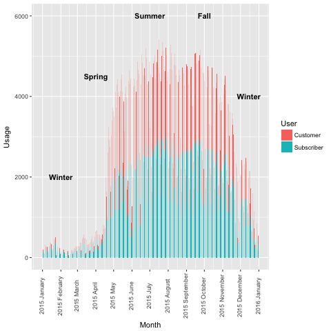
We can see that highest number of trip is in Summer, but wait, there are trips also in Winter! Although, it is not as high as in Winter or Fall. Another fact that we can see from the graph is that more people use the 24-hour or 72-hour pass than becoming monthly or annual member.
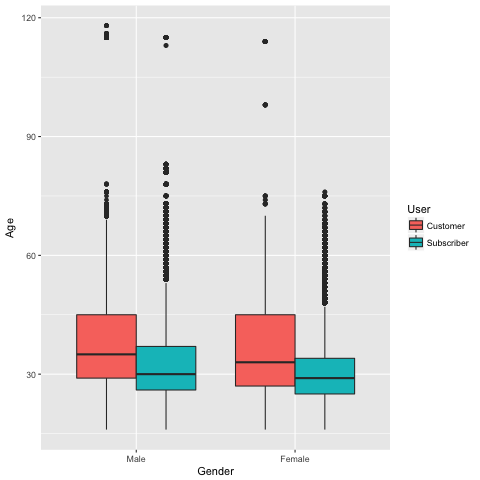
Now, for the last question, how can we understand better the user? One way to answer this is by to know from what age people usually use Hubway, for each membership status and gender. Gender is self-reported by member. We will exclude people who does not provide their gender.
under_30_min_trips %>%
  filter(gender != "Not Provided") %>%
  ggplot +
  geom_boxplot(aes(x = gender, y = age, fill = usertype)) +
  labs(x = "Gender", y = "Age", fill = "User")
Summary
We found many interesting facts laying hidden in our dataset!
Most trip were under 30 minutes
More than 75 % of all trips usually was less than or equal 30 minutes. The most popular station to start with is South Station but Linear Park to Davis Square is the most favourite route (probably because of Somerville bike path?)
Too cold in winter?
As expected, the number of rides dropped during winter. However, some people still rode the bike during the cold. Hubway didn’t close all its stations during winter and it was still possible for some people to ride source. It reached its peak during Summer, and followed by Fall.
30-somethings domination
The average age of short trip riders, regardless their gender and membership status, is around 30 years old.